§ 参考资料 共 6 条
在 3DGS 3. 体渲染 中,我们得到了论文中的体渲染方程:
$$ I_\lambda(\hat{\boldsymbol x})=\int_0^Lc_\lambda(\hat{\boldsymbol x},\xi)g(\hat{\boldsymbol x},\xi)e^{-\int_0^\xi g(\hat{\boldsymbol x},\mu)\mathrm d\mu}\mathrm d\xi $$Splatting 并不是 3DGS 作者提出来的,它来自于论文 Surface splatting,是一种用于点云渲染(Point-Based Rendering)的方法
Surface Splatting
点云本身是对三维场景采样的结果,我们如果要渲染它们,需要对采样点进行重建,得到一个连续的分布,然后再进行渲染
Surface Splatting 用某种连续核函数(如高斯核)去表示每个点的贡献,从而形成一个连续分布
假设我们有一个三维点云表示的场景 $S$,对于三维空间中的任意位置 $\boldsymbol x$,取与它非常相近的一些点 $\{\boldsymbol P_k\}\subset S$,每个点的属性值为 $w_k$,位置为 $\boldsymbol p_k$,核函数为 $r_k(\boldsymbol x)$,那么重建出的分布 $f(\boldsymbol x)$ 表示为:
$$ f(\boldsymbol x)=\sum_{k=0}^Kw_kr_k(\boldsymbol x-\boldsymbol p_k) $$其中,由于每个点都有一个“影响范围”,所以可以看成每个位置只受很相近的点影响,但理论上它受所有点影响
在论文中,由于它探讨的是纹理空间,所以进行了二维参数化,示意图如下:
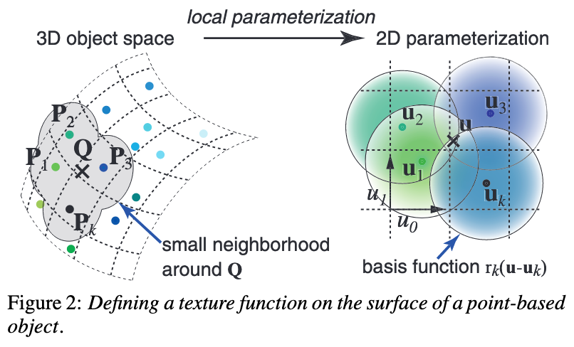
在这个表面上进行重建,原理相似
基于若干假设的 Splatting 算法
我们把颜色看成是离散的(很合理,如果把粒子看成单独个体的话,相邻粒子的颜色完全可以差距很大),而粒子的“密度”是连续的
这样我们根据 Surface Splatting 重建出密度场 $g$,令:
$$ g(\hat{\boldsymbol x},\xi)=\sum_{k=0}^Kg_kr_k(\hat{\boldsymbol x},\xi) $$具体参考 https://zhuanlan.zhihu.com/p/666465701 和 https://zhuanlan.zhihu.com/p/7833648056,代入得到:
$$ \begin{aligned} I_\lambda(\hat{\boldsymbol x})&=\int_0^Lc_\lambda(\hat{\boldsymbol x},\xi)g(\hat{\boldsymbol x},\xi)e^{-\int_0^\xi g(\hat{\boldsymbol x},\mu)\mathrm d\mu}\mathrm d\xi \\ &=\int_0^Lc_\lambda(\hat{\boldsymbol x},\xi)\left(\sum_{k=0}^Kg_kr_k(\hat{\boldsymbol x},\xi)\right)e^{-\int_0^\xi \left(\sum_{k=0}^Kg_kr_k(\hat{\boldsymbol x},\mu)\right)\mathrm d\mu}\mathrm d\xi \\ &=\sum_{k=0}^Kg_k\left(\int_0^Lc_\lambda(\hat{\boldsymbol x},\xi)r_k(\hat{\boldsymbol x},\xi)\prod_{k'=0}^K e^{-g_{k'}\int_0^\xi r_{k'}(\hat{\boldsymbol x},\mu)\mathrm d\mu}\mathrm d\xi\right) \\ &\approx\sum_{k=0}^Kg_k\left[\int_0^Lc_\lambda(\hat{\boldsymbol x},\xi)r_k(\hat{\boldsymbol x},\xi)\prod_{k'=0}^K\left(1-g_{k'}\int_0^\xi r_{k'}(\hat{\boldsymbol x},\mu)\mathrm d\mu\right)\mathrm d\xi\right] \\ &\approx\sum_{k=0}^Kg_k\left(\int_0^Lc_{\lambda k}r_k(\hat{\boldsymbol x},\xi)\mathrm d\xi\right)\prod_{k'=0}^K\left(1-g_{k'}\int_0^L r_{k'}(\hat{\boldsymbol x},\xi)\mathrm d\xi\right) \\ &\approx\sum_{k=0}^Kg_kc_{\lambda k}q_k(\hat{\boldsymbol x})\prod_{k'=0}^{k-1}\left(1-g_{k'}q_{k'}(\hat{\boldsymbol x})\right) \end{aligned} $$这里面有几个重要的近似或假设:
- $e^x\approx 1+x$
- 一个重建核的“能到达相机的概率”($e^\cdot$ 的那部分)只受排在它前面的重建核影响,所以连乘部分只乘到 $k-1$
- 在一个重建核的“支撑域”(影响区域)内,“能到达相机的概率”近似不变,所以可以提出 $\prod$ 部分
- 在一个重建核的“支撑域”内,颜色近似不变
其中,$q_k$ 为重建核沿着轴向的积分,即:
$$ q_k(\hat{\boldsymbol x})=\int_{\mathbb R}r_k(\hat{\boldsymbol x},\xi)\mathrm d\xi $$它被称为足迹函数
如果把高斯作为重建函数的话,3D 高斯沿着某个轴做积分可以得到 2D 高斯,即:
$$ \int_{\mathbb R}\mathcal G_\boldsymbol\Sigma(\boldsymbol x-\boldsymbol\mu)\mathrm dx=\mathcal G_\hat{\boldsymbol\Sigma}(\hat{\boldsymbol x}-\hat{\boldsymbol\mu}) $$其中 $\hat{\boldsymbol\Sigma}$ 就是 $\boldsymbol\Sigma$ 的剩余两维对应的子矩阵,$\hat{\boldsymbol\mu}$ 同理
EWA 重采样算法
要想渲染到一个二维图像中,我们需要将连续的函数 $I_\lambda$ 进行采样来防止走样
最通用的方法是卷上一个低通滤波器 $h$,即:
$$ \begin{aligned} (I_\lambda\otimes h)(\hat{\boldsymbol x})&=\int_{\mathbb R^2}\left[\sum_{k=0}^{K}g_kc_{\lambda k}q_k(\hat{\boldsymbol x})\prod_{k'=0}^{k-1}\left(1-g_{k'}q_{k'}(\hat{\boldsymbol x})\right)\right]h(\hat{\boldsymbol x}-\boldsymbol\mu)\mathrm d\boldsymbol\mu \\ &\approx\int_{\mathbb R^2}\sum_{k=0}^Ko_kg_kc_{\lambda k}q_k(\hat{\boldsymbol x})h(\hat{\boldsymbol x}-\boldsymbol\mu)\mathrm d\boldsymbol\mu \\ &=\sum_{k=0}^Ko_kg_kc_{\lambda k}(q_k\otimes h)(\hat{\boldsymbol x}) \\ &=\sum_{k=0}^Ko_kg_kc_{\lambda k}\rho_k(\hat{\boldsymbol x}) \end{aligned} $$其中,$o_k$ 是累积透明度,这是我们把后面的连乘看作常数得到的,$g_k$ 是当前高斯的不透明度,$c_{\lambda k}$ 是 SH 系数
一般选择 2D 高斯作为滤波函数,如果重建核函数是 3D 高斯的话,这里的卷积就是两个 2D 高斯的卷积,那么两个高斯卷积得到的还是一个高斯,即:
$$ (\mathcal G_{\boldsymbol\Sigma_1}\otimes\mathcal G_{\boldsymbol\Sigma_2})(\boldsymbol x-\boldsymbol\mu)=\mathcal G_{\boldsymbol\Sigma_1+\boldsymbol\Sigma_2}(\boldsymbol x-\boldsymbol\mu) $$在实现上,这里直接对 $q_k$ 对应的协方差矩阵加上 $0.3\boldsymbol I$ 就能得到 $\rho_k$
3DGS 中的渲染方程
3DGS 中使用的渲染方程是这样子的:
$$ C_\lambda(\hat{\boldsymbol x})=\sum_{k=0}^Kc_{\lambda k}g_k\rho_k(\hat{\boldsymbol x})\prod_{k'=0}^{k-1}(1-g_k\rho_k(\hat{\boldsymbol x})) $$即把 $g_k\rho_k(\hat{\boldsymbol x})$ 看作不透明度,然后将累积透明度 $o_k$ 看作是它之前所有高斯的不透明度之和
这与点渲染公式相似:
$$ C_\lambda=\sum_{k=0}^KT_k\alpha_kc_{\lambda k}\quad\text{where}\quad T_k=\prod_{k'=0}^{k-1}(1-\alpha_{k'}) $$3D 高斯的仿射变换
由于 Splatting 是在射线空间中进行的,所以需要把场景中的 3D 高斯变换到射线空间中
从世界空间到相机空间的变换是仿射变换
在 3DGS 1. 高斯分布与高斯椭球 中,我们通过对 $n$ 元标准高斯分布进行推广得到 $n$ 元高斯分布,用了
$$ \boldsymbol Y=\boldsymbol A\boldsymbol X+\boldsymbol\mu $$这个变换,它就是仿射变换
所以,所有的高斯分布都可以看成是标准高斯分布经过仿射变换得到的,高斯分布经过仿射变换后仍然是高斯分布
假设我们有一个高斯分布:
$$ f(\boldsymbol x)=\frac{1}{(2\pi)^{n/2}\vert\boldsymbol\Sigma\vert^{1/2}}e^{-\frac{1}{2}(\boldsymbol x-\boldsymbol \mu)^T\boldsymbol \Sigma^{-1}(\boldsymbol x-\boldsymbol \mu)} $$经过仿射变换 $\boldsymbol y=\varphi(\boldsymbol x)=\boldsymbol A\boldsymbol x+\boldsymbol b$ 后,利用概率密度变换公式得到:
$$ \begin{aligned} f(\boldsymbol y)&=f(\varphi^{-1}(\boldsymbol y))\vert\boldsymbol J\vert \\ &=\frac{1}{(2\pi)^{n/2}\vert\boldsymbol\Sigma\vert^{1/2}}e^{-\frac{1}{2}\left[\boldsymbol A^{-1}(\boldsymbol y-\boldsymbol b)-\boldsymbol\mu\right]^T\boldsymbol\Sigma^{-1}\left[\boldsymbol A^{-1}(\boldsymbol y-\boldsymbol b)-\boldsymbol\mu\right]}\left\vert \boldsymbol A\right\vert^{-1} \\ &=\frac{1}{(2\pi)^{n/2}\vert\boldsymbol\Sigma\vert^{1/2}}e^{-\frac{1}{2}\left[\boldsymbol y-(\boldsymbol A\boldsymbol\mu+\boldsymbol b)\right]^T\boldsymbol(\boldsymbol A\boldsymbol \Sigma\boldsymbol A^T)^{-1}\left[\boldsymbol y-(\boldsymbol A\boldsymbol\mu+\boldsymbol b)\right]}\left\vert \boldsymbol A\right\vert^{-1} \\ &=\frac{1}{(2\pi)^{n/2}\vert\boldsymbol A\boldsymbol \Sigma\boldsymbol A^T\vert^{1/2}}e^{-\frac{1}{2}\left[\boldsymbol y-(\boldsymbol A\boldsymbol\mu+\boldsymbol b)\right]^T\boldsymbol(\boldsymbol A\boldsymbol \Sigma\boldsymbol A^T)^{-1}\left[\boldsymbol y-(\boldsymbol A\boldsymbol\mu+\boldsymbol b)\right]} \end{aligned} $$即:$\boldsymbol\mu'=\boldsymbol A\boldsymbol\mu+\boldsymbol b$,$\boldsymbol\Sigma'=\boldsymbol A\boldsymbol \Sigma\boldsymbol A^T$
3D 高斯的非仿射变换
从相机空间到射线空间的变换是非仿射变换
参考 3DGS 3. 体渲染,对于相机空间中的一个点 $\boldsymbol x$,投影变换函数可以写作:
$$ \phi(\boldsymbol x)=\begin{bmatrix} x_0/x_2 \\ x_1/x_2 \\ \Vert\boldsymbol x\Vert \end{bmatrix} $$我们在将高斯投影到射线空间时,是知道高斯的中心点 $\boldsymbol\mu$ 的,所以我们使用泰勒展开对这个变换进行近似:
$$ \phi(\boldsymbol x)=\phi(\boldsymbol\mu)+\boldsymbol J_{\boldsymbol\mu}(\boldsymbol x-\boldsymbol\mu)+o(\cdot) $$其中,$\boldsymbol J_{\boldsymbol\mu}$ 是 $\phi(\boldsymbol x)$ 对 $\boldsymbol x$ 的一阶导数对应的雅可比矩阵在 $\boldsymbol x=\boldsymbol\mu$ 处的取值,它可以表示成:
$$ \boldsymbol J_{\boldsymbol\mu}=\begin{bmatrix} \frac{\partial \phi_0}{\partial x_0} & \frac{\partial \phi_0}{\partial x_1} & \frac{\partial \phi_0}{\partial x_2} \\ \frac{\partial \phi_1}{\partial x_0} & \frac{\partial \phi_1}{\partial x_1} & \frac{\partial \phi_1}{\partial x_2} \\ \frac{\partial \phi_2}{\partial x_0} & \frac{\partial \phi_2}{\partial x_1} & \frac{\partial \phi_2}{\partial x_2} \end{bmatrix}_{\boldsymbol x=\boldsymbol\mu}=\begin{bmatrix} \frac{1}{x_2} & 0 & -\frac{x_0}{x_2^2} \\ 0 & \frac{1}{x_2} & -\frac{x_1}{x_2^2} \\ \frac{x_0}{\Vert\boldsymbol x\Vert} & \frac{x_1}{\Vert\boldsymbol x\Vert} & \frac{x_2}{\Vert\boldsymbol x\Vert} \end{bmatrix}_{\boldsymbol x=\boldsymbol\mu}=\begin{bmatrix} \frac{1}{\mu_2} & 0 & -\frac{\mu_0}{\mu_2^2} \\ 0 & \frac{1}{\mu_2} & -\frac{\mu_1}{\mu_2^2} \\ \frac{\mu_0}{\Vert\boldsymbol\mu\Vert} & \frac{\mu_1}{\Vert\boldsymbol\mu\Vert} & \frac{\mu_2}{\Vert\boldsymbol\mu\Vert} \end{bmatrix} $$参考 https://zhuanlan.zhihu.com/p/666465701,射线空间的第三维坐标除了取 $\Vert\boldsymbol x\Vert$,也可以取 $x_0$、$x_1$ 或 $x_2$,但是取 $\Vert\boldsymbol x\Vert$ 的效果最好
一阶泰勒展开之后就是仿射变换了,写成:
$$ \phi(\boldsymbol x)\approx\phi(\boldsymbol\mu)+\boldsymbol J_{\boldsymbol\mu}(\boldsymbol x-\boldsymbol\mu)=\boldsymbol J_{\boldsymbol\mu}\boldsymbol x+[\phi(\boldsymbol\mu)-\boldsymbol J_{\boldsymbol\mu}\boldsymbol\mu] $$所以我们可以直接写出:$\boldsymbol\mu'=\phi(\boldsymbol A\boldsymbol\mu+\boldsymbol b)$,$\boldsymbol\Sigma'=\boldsymbol J_{\boldsymbol\mu}\boldsymbol \Sigma\boldsymbol J_{\boldsymbol\mu}^T$
那么,从世界空间到射线空间的变换就是:
$$ \begin{aligned} \boldsymbol\mu'&=\phi(\varphi(\boldsymbol\mu)) \\ \boldsymbol\Sigma'&=\boldsymbol J_{\boldsymbol\mu}\boldsymbol A\boldsymbol \Sigma\boldsymbol A^T\boldsymbol J_{\boldsymbol\mu}^T \end{aligned} $$像素尺度下的投影变换
在转换到射线空间之后,还需要与像素对应起来,3DGS 中使用了焦距,它表示像素尺度上的投影变换比例,可以理解为单位距离跨越了多少像素
假设 $x$ 和 $y$ 方向上的焦距分别为 $f_x$ 与 $f_y$,那么投影变换就可以写成:
$$ \phi(\boldsymbol x)=\begin{bmatrix} f_xx_0/x_2 \\ f_yx_1/x_2 \\ \Vert\boldsymbol x\Vert \end{bmatrix} $$此时雅可比矩阵表示为:
$$ \boldsymbol J_{\boldsymbol\mu}=\begin{bmatrix} f_x\frac{1}{\mu_2} & 0 & -f_x\frac{\mu_0}{\mu_2^2} \\ 0 & f_y\frac{1}{\mu_2} & -f_y\frac{\mu_1}{\mu_2^2} \\ \frac{\mu_0}{\Vert\boldsymbol\mu\Vert} & \frac{\mu_1}{\Vert\boldsymbol\mu\Vert} & \frac{\mu_2}{\Vert\boldsymbol\mu\Vert} \end{bmatrix} $$使用 CUDA 将 3D 高斯转换成 2D 高斯
3D 变换
// Forward method for converting scale and rotation properties of each
// Gaussian to a 3D covariance matrix in world space. Also takes care
// of quaternion normalization.
__device__ void computeCov3D(
    const glm::vec3 scale,              // I  缩放矩阵
    float mod,                          // I  全局放缩
    const glm::vec4 rot,                // I  四元数表示的旋转矩阵
    float* cov3D                        // IO 协方差矩阵(长度为 6,只需存储上三角)
) {
    // Create scaling matrix,缩放矩阵,每个维度都乘上 mod
    glm::mat3 S = glm::mat3(1.0f);
    S[0][0] = mod * scale.x;
    S[1][1] = mod * scale.y;
    S[2][2] = mod * scale.z;

    // Normalize quaternion to get valid rotation
    glm::vec4 q = rot;// / glm::length(rot);
    float r = q.x;
    float x = q.y;
    float y = q.z;
    float z = q.w;

    // Compute rotation matrix from quaternion,从四元数创建旋转矩阵
    glm::mat3 R = glm::mat3(
        1.f - 2.f * (y * y + z * z), 2.f * (x * y - r * z), 2.f * (x * z + r * y),
        2.f * (x * y + r * z), 1.f - 2.f * (x * x + z * z), 2.f * (y * z - r * x),
        2.f * (x * z - r * y), 2.f * (y * z + r * x), 1.f - 2.f * (x * x + y * y)
    );

    // 计算 R^T S^T S R
    glm::mat3 M = S * R;

    // Compute 3D world covariance matrix Sigma
    glm::mat3 Sigma = glm::transpose(M) * M;

    // Covariance is symmetric, only store upper right
    cov3D[0] = Sigma[0][0];
    cov3D[1] = Sigma[0][1];
    cov3D[2] = Sigma[0][2];
    cov3D[3] = Sigma[1][1];
    cov3D[4] = Sigma[1][2];
    cov3D[5] = Sigma[2][2];
}
2D 变换
// Forward version of 2D covariance matrix computation
__device__ float3 computeCov2D(
    const float3& mean,                  // I  世界空间中三维高斯的中心点
    float focal_x, float focal_y,        // I  x、y 两个方向上的焦距
    float tan_fovx, float tan_fovy,      // I  视场角的 tan 值,fov 与 focal 是可以互相计算的
    const float* cov3D,                  // I  世界空间中三维高斯协方差矩阵
    const float* viewmatrix              // I  世界空间到相机空间的转换矩阵(4*4,与传统图形学相同)
) {
    // The following models the steps outlined by equations 29
    // and 31 in "EWA Splatting" (Zwicker et al., 2002).
    // Additionally considers aspect / scaling of viewport.
    // Transposes used to account for row-/column-major conventions.
    float3 t = transformPoint4x3(mean, viewmatrix);           // 得到相机空间中的中心点

    // 将高斯限制在 fov 指定的范围内
    // 前面提到射线空间坐标的前两维可以看成点投影在 z=1 的投影平面内
    // 这里乘上 1.3 而不是 1.0 或者 1.5:
    //   1. 如果太小(1.0),一旦高斯中心稍微越过视锥边界,它会被硬性截到边缘,此时这个高斯在
    //      屏幕上被突然“挤压”;下一帧或梯度更新中它可能又回到视野内,导致闪烁或不连续的梯度
    //   2. 如果太大(1.5),计算量就会变大
    const float limx = 1.3f * tan_fovx;
    const float limy = 1.3f * tan_fovy;
    const float txtz = t.x / t.z;
    const float tytz = t.y / t.z;
    t.x = min(limx, max(-limx, txtz)) * t.z;
    t.y = min(limy, max(-limy, tytz)) * t.z;

    // 雅可比矩阵
    // 由于最后要转换到二维高斯,所以不需要第三行
    glm::mat3 J = glm::mat3(
        focal_x / t.z, 0.0f, -(focal_x * t.x) / (t.z * t.z),
        0.0f, focal_y / t.z, -(focal_y * t.y) / (t.z * t.z),
        0, 0, 0);

    // 取 Y=AX+b 中的 A
    glm::mat3 W = glm::mat3(
        viewmatrix[0], viewmatrix[4], viewmatrix[8],
        viewmatrix[1], viewmatrix[5], viewmatrix[9],
        viewmatrix[2], viewmatrix[6], viewmatrix[10]);

    // J^T W^T S W J
    glm::mat3 T = W * J;

    glm::mat3 Vrk = glm::mat3(
        cov3D[0], cov3D[1], cov3D[2],
        cov3D[1], cov3D[3], cov3D[4],
        cov3D[2], cov3D[4], cov3D[5]);

    glm::mat3 cov = glm::transpose(T) * glm::transpose(Vrk) * T;

    // 转换到像素尺度下的射线空间后,沿轴向积分得到足迹函数对应的 2D 高斯
    // 然后应用低通滤波,协方差矩阵对角线加上 0.3,然后返回

    // Apply low-pass filter: every Gaussian should be at least
    // one pixel wide/high. Discard 3rd row and column.
    cov[0][0] += 0.3f;
    cov[1][1] += 0.3f;

    return { float(cov[0][0]), float(cov[0][1]), float(cov[1][1]) };
}
Tile-Based Rasterizer
在 3DGS 中,使用了基于 Tile 的光栅化,在逐像素光栅化的基础上,将整块屏幕分成若干个 $16\times 16$ 的块,每个高斯只在能“看到”(即在 $3\sigma$ 之内)它的块中渲染
这涉及到 GPU 的 warp 结构,可以加速计算
在前面我们知道,每个高斯会有一个“深度”信息,在这里由于每个高斯被分配到能看到它的 Tile 中,每个这些 Tile 都存在一个该高斯的实例,所以多了一个 Tile 信息,这两个信息组合起来就是高斯的 Key
然后,在渲染的时候按照 Tile、Depth 偏序排序,这样每个 Tile 拥有的高斯可以用一个区间表示,示意图如下:
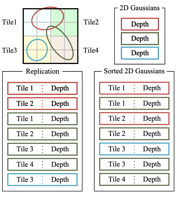
每个 Tile 分配一个线程块,拿到分配到的所有高斯后,再分批对像素进行渲染
在代码中,整个 forward 渲染可以分成两部分:prepross 和 render
预处理
// Perform initial steps for each Gaussian prior to rasterization.
template<int C>
__global__ void preprocessCUDA(
    int P,                                                      // I  高斯的数量
    int D,                                                      // I  球谐函数的维度(0/1/2/3)
    int M,                                                      // I  最大的球谐系数数量,所有高斯的球谐系数都存在一个数组中,用
                                                                //    idx*M 来得到当前高斯的球谐系数
    const float* orig_points,                                   // I  世界坐标系下的所有高斯中心点坐标,长度为 P*3
    const glm::vec3* scales,                                    // I  所有高斯的缩放矩阵对角部分,长度为 P
    const float scale_modifier,                                 // I  全局缩放修正系数
    const glm::vec4* rotations,                                 // I  四元数表示的所有高斯的旋转参数,长度为 P
    const float* opacities,                                     // I  所有高斯的透明度,长度为 P
    const float* shs,                                           // I  所有高斯的球谐系数,长度为 P*M
    bool* clamped,                                              //  O 每个高斯计算完颜色后,如果颜色分量小于 0,那么需要被 clamp,
                                                                //    这个数组记录了每个高斯的颜色分量是否需要 clamp,长度为 P*3
                                                                //    (如果提前计算颜色,那么这里不会输出)
    const float* cov3D_precomp,                                 // I  提前计算的 3D 协方差矩阵(可选),长度为 P*3*3
    const float* colors_precomp,                                // I  提前计算的颜色(可选),长度为 P*3
    const float* viewmatrix,                                    // I  P*4*4
    const float* projmatrix,                                    // I  P*4*4
    const glm::vec3* cam_pos,                                   // I  P
    const int W, int H,                                         // I  宽和高
    const float tan_fovx, float tan_fovy,                       // I
    const float focal_x, float focal_y,                         // I
    int* radii,                                                 //  O 每个高斯在屏幕中的半径,用于给 Tile 分配高斯,长度 P*3
    float2* points_xy_image,                                    //  O 每个高斯在屏幕中的中心点坐标,长度 P
    float* depths,                                              //  O 每个高斯的深度,长度 P
    float* cov3Ds,                                              //  O 每个高斯的 3D 协方差矩阵,是中间结果,长度 P*3*3(如果提前
                                                                //    计算协方差矩阵,那么这里不会输出)
    float* rgb,                                                 //  O 每个高斯的颜色,长度 P*3
    float4* conic_opacity,                                      //  O 每个高斯的屏幕空间 2D 协方差逆矩阵和不透明度,长度 P,协方
                                                                //    差逆矩阵用于快速计算概率密度(参考高斯分布的概率密度函数)
    const dim3 grid,                                            // I  定义坐标系,用于计算 Tile 的覆盖范围
    uint32_t* tiles_touched,                                    //  O 每个高斯覆盖的 Tile 数量,长度 P
    bool prefiltered                                            // I
) {
    // 每个 thread bolck 都计算一个高斯
    auto idx = cg::this_grid().thread_rank();
    if (idx >= P) {
        return;
    }

    // Initialize radius and touched tiles to 0. If this isn't changed,
    // this Gaussian will not be processed further.
    radii[idx] = 0;
    tiles_touched[idx] = 0;

    // Perform near culling, quit if outside.
    // 视锥剔除
    float3 p_view;
    if (!in_frustum(idx, orig_points, viewmatrix, projmatrix, prefiltered, p_view)) {
        return;
    }

    // Transform point by projecting
    // 计算射线空间下的中心点
    float3 p_orig = { orig_points[3 * idx], orig_points[3 * idx + 1], orig_points[3 * idx + 2] };
    float4 p_hom = transformPoint4x4(p_orig, projmatrix);
    float p_w = 1.0f / (p_hom.w + 0.0000001f);
    float3 p_proj = { p_hom.x * p_w, p_hom.y * p_w, p_hom.z * p_w };

    // If 3D covariance matrix is precomputed, use it, otherwise compute
    // from scaling and rotation parameters.
    const float* cov3D;
    if (cov3D_precomp != nullptr) {
        cov3D = cov3D_precomp + idx * 6;
    } else {
        computeCov3D(scales[idx], scale_modifier, rotations[idx], cov3Ds + idx * 6);
        cov3D = cov3Ds + idx * 6;
    }

    // Compute 2D screen-space covariance matrix
    float3 cov = computeCov2D(p_orig, focal_x, focal_y, tan_fovx, tan_fovy, cov3D, viewmatrix);

    // Invert covariance (EWA algorithm)
    // 计算 2D 协方差矩阵的逆矩阵
    float det = (cov.x * cov.z - cov.y * cov.y);
    if (det == 0.0f) {
        return;
    }
    float det_inv = 1.f / det;
    float3 conic = { cov.z * det_inv, -cov.y * det_inv, cov.x * det_inv };

    // Compute extent in screen space (by finding eigenvalues of
    // 2D covariance matrix). Use extent to compute a bounding rectangle
    // of screen-space tiles that this Gaussian overlaps with. Quit if
    // rectangle covers 0 tiles.
    // 特征值分解,拿到缩放矩阵,也就是去除旋转之后的新高斯分布的协方差矩阵
    // 对角线上两个元素就是 sigma,根据 3sigma 原则得到一个半径
    float mid = 0.5f * (cov.x + cov.z);
    float lambda1 = mid + sqrt(max(0.1f, mid * mid - det));
    float lambda2 = mid - sqrt(max(0.1f, mid * mid - det));
    float my_radius = ceil(3.f * sqrt(max(lambda1, lambda2)));

    // 得到屏幕空间中的中心点坐标,并且得到高斯覆盖的矩形范围
    float2 point_image = { ndc2Pix(p_proj.x, W), ndc2Pix(p_proj.y, H) };
    uint2 rect_min, rect_max;
    getRect(point_image, my_radius, rect_min, rect_max, grid);
    if ((rect_max.x - rect_min.x) * (rect_max.y - rect_min.y) == 0) {
        return;
    }

    // If colors have been precomputed, use them, otherwise convert
    // spherical harmonics coefficients to RGB color.
    // 根据球谐系数计算只在当前高斯影响下的相机处的颜色
    if (colors_precomp == nullptr) {
        glm::vec3 result = computeColorFromSH(idx, D, M, (glm::vec3*)orig_points, *cam_pos, shs, clamped);
        rgb[idx * C + 0] = result.x;
        rgb[idx * C + 1] = result.y;
        rgb[idx * C + 2] = result.z;
    }

    // Store some useful helper data for the next steps.
    depths[idx] = p_view.z;
    radii[idx] = my_radius;
    points_xy_image[idx] = point_image;
    // Inverse 2D covariance and opacity neatly pack into one float4
    conic_opacity[idx] = { conic.x, conic.y, conic.z, opacities[idx] };
    tiles_touched[idx] = (rect_max.y - rect_min.y) * (rect_max.x - rect_min.x);
}
渲染之前——分配高斯到 Tile
这里截取 forward 函数的这一部分
主要干的事情就是:
- 拿到每个高斯覆盖 Tile 的数量,然后求前缀和
- 生成 [tile | depth] 表示的 key 和对应的高斯 id 两个数组
- 对这两个数组调用 pairs 排序
- 拿到每个 Tile 在排序后的数组中能看到的 range
...

// Compute prefix sum over full list of touched tile counts by Gaussians
// E.g., [2, 3, 0, 2, 1] -> [2, 5, 5, 7, 8]
//
// 这个函数用法大概是:
// int  num_items;      // e.g., 7
// int  *d_in;          // e.g., [8, 6, 7, 5, 3, 0, 9]
// int  *d_out;         // e.g., [ ,  ,  ,  ,  ,  ,  ]
//
// cub::DeviceScan::InclusiveSum(d_temp_storage, temp_storage_bytes, d_in, d_out, num_items);
//
// d_out <-- [8, 14, 21, 26, 29, 29, 38]
// 也就是求一个前缀和
CHECK_CUDA(cub::DeviceScan::InclusiveSum(
    geomState.scanning_space,
    geomState.scan_size,
    geomState.tiles_touched,
    geomState.point_offsets,
    P), debug)

// Retrieve total number of Gaussian instances to launch and resize aux buffers
// 从显存中拿出总数,等会要返回
int num_rendered;
CHECK_CUDA(cudaMemcpy(&num_rendered, geomState.point_offsets + P - 1, sizeof(int), cudaMemcpyDeviceToHost), debug);

size_t binning_chunk_size = required<BinningState>(num_rendered);
char* binning_chunkptr = binningBuffer(binning_chunk_size);
BinningState binningState = BinningState::fromChunk(binning_chunkptr, num_rendered);

// For each instance to be rendered, produce adequate [ tile | depth ] key
// and corresponding dublicated Gaussian indices to be sorted
// 根据 Tile 覆盖情况生成 [ tile | depth ] key 和高斯 id 两个列表
duplicateWithKeys<<<(P + 255) / 256, 256>>>(
    P,
    geomState.means2D,
    geomState.depths,
    geomState.point_offsets,
    binningState.point_list_keys_unsorted,
    binningState.point_list_unsorted,
    radii,
    tile_grid)

// 表示所以 tile 所需要的位数
int bit = getHigherMsb(tile_grid.x * tile_grid.y);

// Sort complete list of (duplicated) Gaussian indices by keys
// 把 point_list_keys_unsorted 和 point_list_unsorted 总共 num_rendered 项
// 按照 key 的第 0 到 32 + bit(左开右闭)排序,结果放到对应的新数组中
CHECK_CUDA(cub::DeviceRadixSort::SortPairs(
    binningState.list_sorting_space,
    binningState.sorting_size,
    binningState.point_list_keys_unsorted, binningState.point_list_keys,
    binningState.point_list_unsorted, binningState.point_list,
    num_rendered, 0, 32 + bit), debug)

CHECK_CUDA(cudaMemset(imgState.ranges, 0, tile_grid.x * tile_grid.y * sizeof(uint2)), debug);

// Identify start and end of per-tile workloads in sorted list
if (num_rendered > 0) {
    // 根据 point_list_keys 总共 num_rendered 项拿到每个 Tile 的用下标区间表示的所有高斯
    // 并且放到 ranges(uint2* 类型)中
    identifyTileRanges<<<(num_rendered + 255) / 256, 256>>>(
        num_rendered,
        binningState.point_list_keys,
        imgState.ranges);
}

...
渲染
// Main rasterization method. Collaboratively works on one tile per
// block, each thread treats one pixel. Alternates between fetching
// and rasterizing data.
// GPU 有 grid、block、thread 三层结构,每层结构都有一个二维的 index,来映射图像数据
// 渲染的时候,图像大小是 W*H,那么:
//   grid 有 W/16 * H/16 个 block
//   block 有 16 * 16 个 tread
// 一个 thread 就表示一个像素,一个 block 表示一个 Tile
// 这里把一个 thread 既用来处理像素,又用来读取高斯
template <uint32_t CHANNELS>                             // 通道数,这里就是 RGB 三个通道
__global__ void __launch_bounds__(BLOCK_X * BLOCK_Y)     // 每个 Tile 内部渲染像素时的最大线程数,这里就是 16*16
renderCUDA(
    const uint2* __restrict__ ranges,                    // I  每个 Tile 对应的区间
    const uint32_t* __restrict__ point_list,             // I  所有的高斯
    int W, int H,                                        // I  屏幕的宽和高
    const float2* __restrict__ points_xy_image,          // I  每个高斯的中心点
    const float* __restrict__ features,                  // I  每个高斯的特征,与 CHANNELS 相对应,长度 P*CHANNELS
    const float4* __restrict__ conic_opacity,            // I  每个高斯的协方差逆矩阵以及不透明度,长度 P
    float* __restrict__ final_T,                         //  O 最后每个像素的透射率(即背景色的权重),长度 W*H
    uint32_t* __restrict__ n_contrib,                    //  O 最后每个像素的对该像素产生贡献的高斯数量,长度 W*H
    const float* __restrict__ bg_color,                  // I  背景色,长度 CHANNELS
    float* __restrict__ out_color                        //  O 输出颜色,长度 W*H*CHANNELS
) {
    // Identify current tile and associated min/max pixel range.
    // 算出当前 thread block 代表的 Tile 的范围(pix_min 和 pix_max)和 ID
    // 以及当前 thread 代表的像素
    auto block = cg::this_thread_block();
    uint32_t horizontal_blocks = (W + BLOCK_X - 1) / BLOCK_X;
    uint2 pix_min = { block.group_index().x * BLOCK_X, block.group_index().y * BLOCK_Y };
    uint2 pix_max = { min(pix_min.x + BLOCK_X, W), min(pix_min.y + BLOCK_Y , H) };
    uint2 pix = { pix_min.x + block.thread_index().x, pix_min.y + block.thread_index().y };
    uint32_t pix_id = W * pix.y + pix.x;
    float2 pixf = { (float)pix.x, (float)pix.y };

    // Check if this thread is associated with a valid pixel or outside.
    bool inside = pix.x < W && pix.y < H;
    // Done threads can help with fetching, but don't rasterize
    // 如果不在屏幕内,那么直接标记结束
    bool done = !inside;

    // Load start/end range of IDs to process in bit sorted list.
    // 每个线程既负责对像素进行光栅化,也负责读取高斯信息,所以读取的高斯数量 BLOCK_SIZE(也就是 BLOCK_X * BLOCK_Y)
    // 与线程数量相同,每个线程先进行把高斯都拿到放到共享内存中,同步后利用读到的高斯对每个像素进行光栅化
    uint2 range = ranges[block.group_index().y * horizontal_blocks + block.group_index().x];
    const int rounds = ((range.y - range.x + BLOCK_SIZE - 1) / BLOCK_SIZE);
    int toDo = range.y - range.x;

    // Allocate storage for batches of collectively fetched data.
    // thread block 内共享的变量,读取到的高斯数据
    __shared__ int collected_id[BLOCK_SIZE];
    __shared__ float2 collected_xy[BLOCK_SIZE];
    __shared__ float4 collected_conic_opacity[BLOCK_SIZE];

    // Initialize helper variables
    float T = 1.0f;
    uint32_t contributor = 0;
    uint32_t last_contributor = 0;
    float C[CHANNELS] = { 0 };

    // Iterate over batches until all done or range is complete
    for (int i = 0; i < rounds; i++, toDo -= BLOCK_SIZE) {
        // End if entire block votes that it is done rasterizing
        // 所用线程同步到这个位置,并且统计所有线程中已经光栅化的像素数量,如果全部光栅化完成,那么 break
        // 这算是一个剪枝
        int num_done = __syncthreads_count(done);
        if (num_done == BLOCK_SIZE) {
            break;
        }

        // Collectively fetch per-Gaussian data from global to shared
        // block.thread_rank() 返回在 block 内 thread 的线性编号
        // 读取这个线程需要读的高斯
        int progress = i * BLOCK_SIZE + block.thread_rank();
        if (range.x + progress < range.y) {
            int coll_id = point_list[range.x + progress];
            collected_id[block.thread_rank()] = coll_id;
            collected_xy[block.thread_rank()] = points_xy_image[coll_id];
            collected_conic_opacity[block.thread_rank()] = conic_opacity[coll_id];
        }

        // 同步
        block.sync();

        // Iterate over current batch
        // 用读到的高斯对当前线程代表的像素进行光栅化
        for (int j = 0; !done && j < min(BLOCK_SIZE, toDo); j++) {
            // Keep track of current position in range
            contributor++;

            // Resample using conic matrix (cf. "Surface
            // Splatting" by Zwicker et al., 2001)
            // 计算 2D 高斯概率密度函数中的指数部分
            float2 xy = collected_xy[j];
            float2 d = { xy.x - pixf.x, xy.y - pixf.y };
            float4 con_o = collected_conic_opacity[j];
            float power = -0.5f * (con_o.x * d.x * d.x + con_o.z * d.y * d.y) - con_o.y * d.x * d.y;
            if (power > 0.0f) {
                // 正常情况下这里一定是大于 0 的,如果不是,那么一定有异常,直接跳过
                continue;
            }

            // Eq. (2) from 3D Gaussian splatting paper.
            // Obtain alpha by multiplying with Gaussian opacity
            // and its exponential falloff from mean.
            // Avoid numerical instabilities (see paper appendix).
            // 计算 g_k*rho_k,高斯概率密度函数中的系数被合并到了 g_k 中进行学习
            float alpha = min(0.99f, con_o.w * exp(power));
            if (alpha < 1.0f / 255.0f) {
                continue;
            }
            float test_T = T * (1 - alpha);
            if (test_T < 0.0001f) {
                // 这里是一个剪枝,如果剩余透射率非常小,认为像素已经几乎被完全覆盖,跳过
                // 这里不加上当前高斯的贡献是因为之后会加上背景色
                done = true;
                continue;
            }

            // Eq. (3) from 3D Gaussian splatting paper.
            for (int ch = 0; ch < CHANNELS; ch++) {
                // 渲染公式
                C[ch] += features[collected_id[j] * CHANNELS + ch] * alpha * T;
            }

            // T_k=T_{k-1}*(1-alpha_k)
            T = test_T;

            // Keep track of last range entry to update this
            // pixel.
            last_contributor = contributor;
        }
    }

    // All threads that treat valid pixel write out their final
    // rendering data to the frame and auxiliary buffers.
    if (inside) {
        final_T[pix_id] = T;
        n_contrib[pix_id] = last_contributor;
        for (int ch = 0; ch < CHANNELS; ch++) {
            out_color[ch * H * W + pix_id] = C[ch] + T * bg_color[ch];
        }
    }
}